Showing posts with label storms. Show all posts

Wednesday, January 30, 2019

A Revision of Future Climate Change Trends

By Andrew Glikson

Abstract


As the Earth continues to heat, paleoclimate evidence suggests transient reversals will result in accentuating the temperature polarities, leading to increase in the intensity and frequency of extreme weather events.

Pleistocene paleoclimate records indicate interglacial temperature peaks are consistently succeeded by transient stadial freeze events, such as the Younger Dryas and the 8.5 kyr-old Laurentide ice melt, attributed to cold ice melt water flow from the polar ice sheets into the North Atlantic Ocean. The paleoclimate evidence raises questions regarding the mostly linear to curved future climate model trajectories proposed for the 21ᵗʰ century and beyond, not marked by tipping points. However, early stages of a stadial event are manifest by a weakening of the North Atlantic overturning circulation and the build-up of a large pool of cold water south and east of Greenland and along the fringes of Western Antarctica. Comparisons with climates of the early Holocene Warm Period and the Eemian interglacial when global temperatures were about +1°C higher than late Holocene levels. The probability of a future stadial event bears major implications for modern and future climate change trends, including transient cooling of continental regions fringing the Atlantic Ocean, an increase in temperature polarities between polar and tropical zones across the globe, and thereby an increase in storminess, which need to be taken into account in planning global warming adaptation efforts.

Introduction

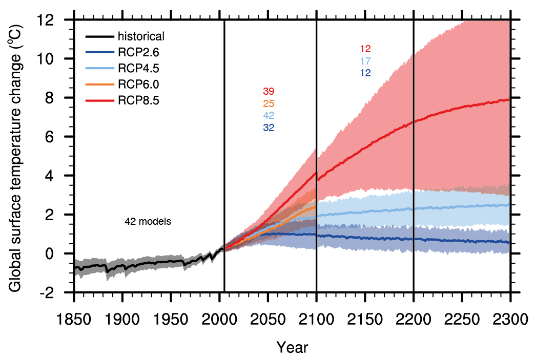
Reports of the International Panel of Climate Change (IPCC)⁽¹⁾, based on thousands of peer reviewed science papers and reports, offer a confident documentation of past and present processes in the atmosphere⁽²⁾, including future model projections (Figure 1). When it comes to estimates of future ice melt and sea level change rates, however, these models contain a number of significant departures from observations based on the paleoclimate evidence, from current observations and from likely future projections. This includes departures in terms of climate change feedbacks from land and water, ice melt rates, temperature trajectories, sea level rise rates, methane release rates, the role of fires, and observed onset of transient stadial (freeze) events⁽³⁾. Early stages of stadial event/s are manifest by the build-up of a large pool of cold water in the North Atlantic Ocean south of Greenland and along the fringes of the Antarctic continent (Figure 2).
Figure 1. IPCC AR5: Time series of global annual mean surface air temperature anomalies relative to 1986–2005
from CMIP5 (Coupled Model Inter-comparison Project) concentration-driven experiments.
Projections are shown for each RCP for the multi model mean (solid lines) and the 5–95%
range (±1.64 standard deviation) across the distribution of individual models (shading).⁽⁴⁾
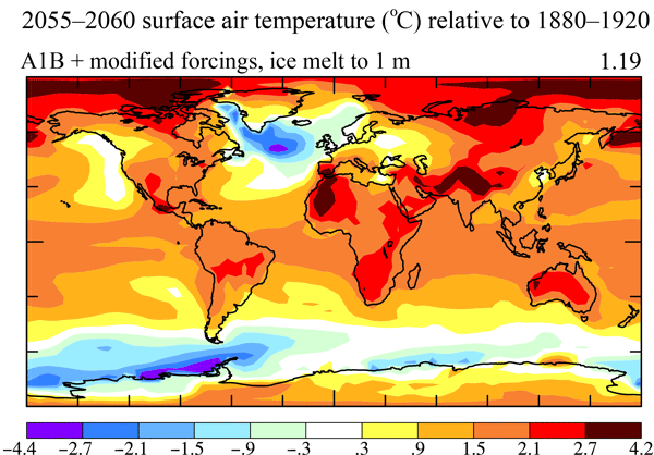
Hansen et al. (2016) (Figure 2) used paleoclimate data and modern observations to estimate the effects of ice melt water from Greenland and Antarctica, showing cold low-density meltwater tend to cap increasingly warm subsurface ocean water, affecting an increase ice shelf melting, accelerating ice sheet mass loss (Figure 3) and slowing of deep water formation (Figure 4). Ice mass loss would raise sea level by several meters in an exponential rather than linear response, with doubling time of ice loss of 10, 20 or 40 years yielding multi-meter sea level rise in about 50, 100 or 200 years.

Linear to curved temperature trends portrayed by the IPCC to the year 2300 (Figure 1) are rare in the Pleistocene paleo-climate record, which abrupt include warming and cooling variations during both glacial (Dansgaard-Oeschger cycles; Ganopolski and Rahmstorf 2001⁽⁵⁾; Camille and Born, 2019⁽⁶⁾) and interglacial (Cortese et al. 2007⁽⁷⁾) periods. Hansen et al.’s (2016) model includes sharp drops in temperature, reflecting stadial freezing events in the Atlantic Ocean and the sub-Antarctic Ocean and their surrounds, reaching -2°C over several decades (Figure 5).
Figure 2. 2055-2060 surface-air temperature to +1.19°C above 1880-1920
(AIB model modified forcing, ice melt to 1 meter) From: Hansen et al. (2016)⁽⁸⁾
Figure 3. Greenland and Antarctic ice mass change. GRACE data are extension of Velicogna et al. (2014)⁽⁹⁾
gravity data. MBM (mass budget method) data are from Rignot et al. (2011)⁽¹⁰⁾. Red curves are gravity
data for Greenland and Antarctica only; small Arctic ice caps and ice shelf melt add to freshwater input.⁽¹¹⁾
Figure 4. (a) AMOC (Sverdrup⁽¹²⁾) at 28°N in simulations (i.e., including freshwater injection of 720 Gt year−1 in 2011
                around Antarctica, increasing with a 10-year doubling time, and half that amount around Greenland).
(b) SST (°C) in the North Atlantic region (44–60°N, 10–50°W).
Temperature and sea level rise relations during the Eemian interglacial⁽¹³⁾ about 115-130 kyr ago, when temperatures were about +1°C or higher than during the late stage of the Holocene, and sea levels were +6 to +9 m higher than at present, offer an analogy for present developments. During the Eemian overall cooling of the North Atlantic Ocean and parts of the West Antarctic fringe ocean due to ice melt led to increased temperature polarities and to storminess⁽¹⁴⁾, underpinning the danger of global temperature rise to +1.5°C. Accelerating ice melt and nonlinear sea level rise would reach several meters over a timescale of 50–150 years (Hansen et al. 2016)

Figure 5. Global surface-air temperature to the year 2300 in the North Atlantic and Southern Oceans,
including stadial freeze events as a function of Greenland and Antarctic ice melt doubling time

Portents of collapse of the Atlantic Meridional Ocean Circulation (AMOC)


The development of large cold water pools south and east of Greenland (Rahmstorf et al. 2015⁽¹⁵⁾) and at the fringe of West Antarctica (Figures 1 and 5) signify early stages in the development of a stadial, consistent with the decline in the Atlantic Meridional Ocean Circulation (AMOC) (Figure 4). These projections differ markedly from linear model trends (Figure 1). IPCC models mainly assume long term ice melt⁽¹⁶⁾, stating “For the 21st century, we expect that surface mass balance changes will dominate the volume response of both ice sheets (Greenland and Antarctica). A key question is whether ice-dynamical mechanisms could operate which would enhance ice discharge sufficiently to have an appreciable additional effect on sea level rise”⁽¹⁷⁾. The IPCC conclusion is difficult to reconcile with studies by Rignot et al. (2011) reporting that in 2006 the Greenland and Antarctic ice sheets experienced a “combined mass loss of 475 ± 158 Gt/yr, equivalent to 1.3 ± 0.4 mm/yr sea level rise”⁽¹⁸⁾. For the Antarctic ice sheet the IEMB team (2017) states the sheet lost 2,720 ± 1,390 billion tonnes of ice between 1992 and 2017, which corresponds to an increase in mean sea level of 7.6 ± 3.9 millimeter⁽¹⁹⁾.

A non-linear climate warming trend, including stadial freeze events, bears significant implications for planning future adaptation efforts, including preparations for transient deep freeze events in parts of Western Europe and eastern North America, for periods lasting several decades (Figure 5) and coastal defenses against enhanced storminess arising from increased temperature contrasts between the cooled regions and warm tropical latitudes.

Imminent climate risks

Climate model projections for the 21ᵗʰ to 23ʳᵈ centuries need to take paleoclimate evidence more fully into account, including the transient stadial effects of ice melt water flow into the oceans and amplifying feedbacks of global warming from land and oceans. Radiative forcing⁽²⁰], increasing with concentration of atmospheric greenhouse gases and rising by about 0.04 Watt/m²/year over the last 50 years⁽²¹⁾, totaled by more than 2 Watt/m², equivalent to ~3.0°C (~1.5°C per W/m²)⁽²²⁾. The rise of mean global temperatures to date by 0.9°C since 1880⁽²³⁾ therefore represents lag effect, pointing to potential temperature rise by approximately two degrees Celsius. A further rise in global temperatures would be enhanced by amplifying feedbacks from land and oceans, including exposure of water surfaces following sea ice melting, reduction of CO₂ concentration in water, release of methane and fires. Climate change trajectories would be highly irregular as a result of stadial events affected by flow of ice melt water into the oceans. Whereas similar temperature fluctuations and stadial events occurred during past interglacial periods (Cortese et al. 2007⁽²⁴⁾; Figure 6), when temperature fluctuations were close to ~1°C, further rises in temperature in future would enhance the intensity and frequency of extreme weather events, entering uncharted territory unlike any recorded during the Pleistocene, rendering large parts of the continents uninhabitable.

Figure 6. (A) Evolution of sea surface temperatures in 5 glacial-interglacial transitions recorded in ODP 1089
at the sub-Antarctic Atlantic Ocean. Lower grey lines – δ¹⁸O measured on Cibicidoides plankton;
Black lines – sea surface temperature. Marine isotope stage numbers are indicated on top of diagrams.
Note the stadial temperature drop events following interglacial peak temperatures, analogous
to the Younger Dryas preceding the onset of the Holocene (Cortese et al. 2007⁽²⁵⁾).
(B) Mean temperatures for the late Pleistocene and early Holocene.

Note to readers: please click the share buttons above. Forward this article to your email lists. 
Crosspost on your blog site, internet forums. etc.

Andrew Glikson
by Andrew Glikson
Earth and Paleo-climate science, Australia National University (ANU) School of Anthropology and Archaeology,
ANU Planetary Science Institute,
ANU Climate Change Institute,
Honorary Associate Professor, Geothermal Energy Centre of Excellence, University of Queensland.

Books:
http://www.springer.com/gp/book/9783319079073
http://www.springer.com/gp/book/9789400763272
http://www.springer.com/us/book/9783319745442
http://www.springer.com/gp/book/9783319225111
http://www.springer.com/gp/book/9783319572369
http://www.springer.com/gp/book/9789400773318


Notes

(1) IPCC, Special Report, Global Warming of 1.5 ºC
https://www.ipcc.ch
https://www.ipcc.ch/sr15/

(2) Climate Council, Report, The good, the bad and the ugly: limiting temperature rise to 1.5°C
https://www.climatecouncil.org.au/resources/limiting-temperature-rise/

(3) Ice melt, sea level rise and superstorms: evidence from paleoclimate data, climate modeling, and modern observations that 2 °C global warming could be dangerous, by James Hansen et al.
https://www.atmos-chem-phys.net/16/3761/2016/

(4) IPCC Climate Change 2013: Technical Summary, p.89
http://www.climatechange2013.org/images/figures/WGI_AR5_Fig12-5.jpg
http://www.climatechange2013.org/images/report/WG1AR5_TS_FINAL.pdf

(5) Rapid changes of glacial climate simulated in a coupled climate model, by Andrey Ganopolski and Stefan Rahmstorf
https://www.nature.com/articles/35051500
https://www.ncbi.nlm.nih.gov/pubmed/11196631

(6) Coupled atmosphere-ice-ocean dynamics in Dansgaard-Oeschger events, by Camille Li and Andreas Born
https://www.sciencedirect.com/science/article/pii/S0277379118305705

(7) The last five glacial‐interglacial transitions: A high‐resolution 450,000‐year record from the subantarctic Atlantic, by G. Cortese, A. Abelmann and R. Gersonde
https://agupubs.onlinelibrary.wiley.com/doi/full/10.1029/2007PA001457

(8) Ice melt, sea level rise and superstorms: evidence from paleoclimate data, climate modeling, and modern observations that 2 °C global warming could be dangerous, by James Hansen et al. (2016)
https://www.atmos-chem-phys.net/16/3761/2016/acp-16-3761-2016-avatar-web.png
https://www.atmos-chem-phys.net/16/3761/2016/

(9) Regional acceleration in ice mass loss from Greenland and Antarctica using GRACE time‐variable gravity data, by I. Velicogna et al.
https://agupubs.onlinelibrary.wiley.com/doi/10.1002/2014GL061052

(10) Acceleration of the contribution of the Greenland and Antarctic ice sheets to sea level rise, by E. Rignot et al. (2011)
https://agupubs.onlinelibrary.wiley.com/doi/10.1029/2011GL046583

(11) Ice melt, sea level rise and superstorms: evidence from paleoclimate data, climate modeling, and modern observations that 2 °C global warming could be dangerous, by James Hansen et al.
https://www.atmos-chem-phys.net/16/3761/2016/acp-16-3761-2016.pdf

(12) Sverdrup: Unit of flow – 1 Sv is equal to 1,000,000 m³ per second
https://en.wikipedia.org/wiki/Sverdrup

(13) Eemian Interglacial Stage
https://www.britannica.com/science/Eemian-Interglacial-Stage

(14) Giant boulders and Last Interglacial storm intensity in the North Atlantic, by Alessio Rovere et al. (2017)
http://moraymo.us/wp-content/uploads/2018/03/Rovereetal_PNAS_2017.pdf
Northern hemisphere winter storm tracks of the Eemian interglacial and the last glacial inception, by F. Kaspar (2006)
https://www.clim-past.net/3/181/2007/cp-3-181-2007.pdf

(15) Exceptional twentieth-century slowdown in Atlantic Ocean overturning circulation, by Stefan Rahmstorf et al. (2015)
https://www.nature.com/articles/nclimate2554

(16) The UN's Devastating Climate Change Report Was Too Optimistic, by Nafeez Ahmed (Oct 16, 2018)
https://motherboard.vice.com/en_us/article/43e8yp/the-uns-devastating-climate-change-report-was-too-optimistic

(17) IPCC Third Assessment Report, Working Group I: The Scientific Basis
https://archive.ipcc.ch/ipccreports/tar/wg1/416.htm

(18) Acceleration of the contribution of the Greenland and Antarctic ice sheets to sea level rise, by E. Rignot et al. (2011)
https://agupubs.onlinelibrary.wiley.com/doi/full/10.1029/2011GL046583

(19) Mass balance of the Antarctic Ice Sheet from 1992 to 2017
https://www.nature.com/articles/s41586-018-0179-y.epdf

(20) Radiative forcing – the difference between incoming radiation and radiation reflected back to space
https://en.wikipedia.org/wiki/Radiative_forcing

(21) Climate Change in a Nutshell: The Gathering Storm, by James Hansen (18 December 2018)
http://www.columbia.edu/~jeh1/mailings/2018/20181206_Nutshell.pdf

(22) Target atmospheric CO2: Where should humanity aim?, by James Hansen (2008)
https://arxiv.org/abs/0804.1126

(23) NASA: Global temperature
https://climate.nasa.gov/vital-signs/global-temperature/

(24) The last five glacial‐interglacial transitions: A high‐resolution 450,000‐year record from the subantarctic Atlantic, by G. Cortese, A. Abelmann and R. Gersonde
https://agupubs.onlinelibrary.wiley.com/doi/full/10.1029/2007PA001457

(25) The last five glacial‐interglacial transitions: A high‐resolution 450,000‐year record from the subantarctic Atlantic, by G. Cortese, A. Abelmann and R. Gersonde
https://agupubs.onlinelibrary.wiley.com/doi/full/10.1029/2007PA001457

This is an edited version of an article at Global Research
Copyright © Dr. Andrew Glikson, 2019

Sunday, January 20, 2019

Care for the Ozone Layer


The stratosphere normally is cold and very dry. Global warming can increase water vapor in the stratosphere in a number of ways. Global warming causes the troposphere to warm and since warmer air holds more water vapor, the amount of water vapor in the troposphere is increasing. This can cause more water vapor to end up in the stratosphere as well, as described below.

Stratospheric Water Vapor over the Arctic

Around the time of the December Solstice, very little sunlight is reaching the Arctic and temperatures over land at higher latitudes can get very low. At the same time, global warming has made oceans warmer and this keeps air temperatures over water relatively warm in Winter. This can lead to a number of phenomena including sudden stratospheric warming and moistening of the stratosphere.

Sudden stratospheric warming is illustrated by the image on the right, showing temperatures in the stratosphere over Siberia as high as 12.7°C or 54.9°F on December 24, 2018, and temperatures as low as -84.8°C or -120.6°F over Greenland.

At the same time, relative humidity was as high as 100% in the stratosphere over the North Sea, as the second image on the right shows.

Moistening of the stratosphere was even more pronounced on December 24, 2016, as illustrated by the third image on the right.

Storms over the U.S.

Jennifer Francis has long pointed out that, as temperatures at the North Pole are rising faster than at the Equator, the Jet Stream is becoming wavier and can get stuck in a 'blocking pattern' for days, increasing the duration and intensity of extreme weather events.

This can result in stronger storms moving more water vapor inland over the U.S., and such storms can cause large amounts of water vapor to rise high up in the sky.

Water vapor reaching stratospheric altitudes causes loss of ozone, as James Anderson describes in a 2017 paper and discusses in the short 2016 video below.


Methane

Stratospheric water vapor can also result from methane oxidation in the stratosphere. Methane concentrations have risen strongly at higher altitudes over the years. Noctilucent clouds indicate that methane has led to water vapor in the upper atmosphere.

The danger is that, as the Arctic Ocean keeps warming, large eruptions of methane will occur from the seafloor. Ominously, high methane levels have recently shown up on satellite images over the Arctic at lower altitudes, indicating the methane is escaping from the sea.

The images below show methane levels recorded by the NPP satellite:
Jan. 6, 2019, with peak levels of 2513 ppb at 1000 mb, 2600 ppb at 840 mb and 2618 ppb at 695 mb;
Jan. 11, 2019, with peak levels of 2577 ppb at 1000 mb, 2744 ppb at 840 mb and 2912 ppb at 695 mb;
Jan. 15, 2019, with peak levels of 2524 ppb at 1000 mb, 2697 ppb at 840 mb and 2847 ppb at 695 mb.


The images below show methane levels recorded by the MetOp satellites:
Jan. 15, 2019, with peak levels of 2177 ppb at 840 mb, 2342 ppb at 695 mb and 2541 ppb at 586 mb;
Jan. 16, 2019, with peak levels of 2219 ppb at 840 mb, 2299 ppb at 695 mb and 2475 ppb at 586 mb;
Jan. 19, 2019, with peak levels of 2201 ppb at 840 mb, 2489 ppb at 695 mb and 2813 ppb at 586 mb.


The Importance of the Ozone Layer

Increases in stratospheric water vapor are bad news, as they speed up global warming and lead to loss of stratospheric ozone, as Drew Shindell pointed out back in 2001.

It has long been known that deterioration of the ozone shield increases ultraviolet-B irradiation, in turn causing skin cancer. Recent research suggest that, millions of years ago, it could also have led to loss of fertility and consequent extinction in plants and animals (see box right).

Nitrous oxide

As the left panel of the image below shows, growth in the levels of chlorofluorocarbons (CFCs) has slowed over the years, but their impact will continue for a long time, given their long atmospheric lifetime (55 years for CFC-11 and 140 years for CFC-12, CCl2F2).

Furthermore, as the right panel shows, the impact of nitrous oxide (N₂O) as an ozone depleting substance (ODS) has relatively grown, while N₂O levels also continue to increase in the atmosphere.

[ click on images to enlarge ]
Existential Threats

In conclusion, rising levels of emissions by people constitute existential threats in many ways. Rising temperatures cause heat stress and infertility, and there are domino effects. Furthermore, stratospheric ozone loss causes cancer and infertility.

Only once the ozone layer formed on Earth some 600 million years ago could multicellular life develop and survive. Further loss of stratospheric ozone could be the fastest path to extinction for humanity, making care for the ozone layer imperative.

As described in an earlier post, Earth is on the edge of runaway warming and in a moist-greenhouse scenario oceans evaporate into the stratosphere with loss of the ozone layer.

The situation is dire and calls for comprehensive and effective action, as described in the Climate Plan.


Links

• Climate and ozone response to increased stratospheric water vapor, by Drew Shindell (2001)
https://agupubs.onlinelibrary.wiley.com/doi/abs/10.1029/1999GL011197

• Stratospheric ozone over the United States in summer linked to observations of convection and temperature via chlorine and bromine catalysis, by James Anderson et al. (2017)
https://www.pnas.org/content/114/25/E4905

• Harvard Speaks on Climate Change: James Anderson (2016)
https://vimeo.com/185794598

• Climate Week: Climate Science Breakfast with James Anderson (April 9, 2015)
http://environment.harvard.edu/climate-week-climate-science-breakfast-james-anderson

• 10°C or 18°F warmer by 2021?
https://arctic-news.blogspot.com/2017/04/10c-or-18f-warmer-by-2021.html

• Noctilucent clouds indicate more methane in upper atmosphere
https://arctic-news.blogspot.com/2012/09/noctilucent-clouds-indicate-more-methane-in-upper-atmosphere.html

• Noctilucent clouds: further confirmation of large methane releases
https://methane-hydrates.blogspot.com/2013/12/noctilucent-clouds-further-confirmation-of-large-methane-releases.html

• It could be unbearably hot in many places within a few years time
https://arctic-news.blogspot.com/2016/07/it-could-be-unbearably-hot-in-many-places-within-a-few-years-time.html

• Climate change: effect on sperm could hold key to species extinction, by Kris Sales
https://theconversation.com/climate-change-effect-on-sperm-could-hold-key-to-species-extinction-107375

• Climate change: effect on sperm could hold key to species extinction
https://theconversation.com/climate-change-effect-on-sperm-could-hold-key-to-species-extinction-107375

• UV-B–induced forest sterility: Implications of ozone shield failure in Earth’s largest extinction, by Jeffrey Benca et al. (2018)
http://advances.sciencemag.org/content/4/2/e1700618

• Co-extinctions annihilate planetary life during extreme environmental change, by Giovanni Strona and Corey Bradshaw (2018)
https://www.nature.com/articles/s41598-018-35068-1

• NOAA's Annual Greenhouse Gas Index
https://www.esrl.noaa.gov/gmd/aggi

• NOAA Study Shows Nitrous Oxide Now Top Ozone-Depleting Emission
https://www.esrl.noaa.gov/news/2009/nitrous_oxide_top_ozone_depleting_gas.html

• Earth is on the edge of runaway warming
https://arctic-news.blogspot.com/2013/04/earth-is-on-the-edge-of-runaway-warming.html

• Climate Plan
https://arctic-news.blogspot.com/p/climateplan.html


Monday, October 2, 2017

The Arctic is Changing the Jet Stream - Why This Is Important

By Sam Carana, with contributions by Jennifer Francis

Global warming is increasing the strength of hurricanes. A warmer atmosphere holds more water vapor and sea surface temperatures are rising. Both of these changes strengthen hurricanes. Steering winds may also be changing, causing unusual hurricane tracks such as Sandy's left turn into the mid-Atlantic seaboard and Harvey's stagnation over Houston. Is rapid Arctic warming playing a role?

Jennifer Francis has long been warning that global warming is increasing the likelihood of wavier jet stream patterns and more frequent blocking events, both of which have been observed. The Arctic is warming more rapidly than the rest of the world. The narrowing temperature difference between the Arctic and lower latitudes is weakening the speed at which the jet stream circumnavigates Earth and may be making the jet stream more wavy. In a 2012 study, Jennifer Francis and Stephen Vavrus warned that this makes atmospheric blocking events in the Northern Hemisphere more likely, aggravating extreme weather events related to stagnant weather conditions, such as drought, flooding, cold spells, and heat waves.

The danger was highlighted later that year, when a strong block associated with a deep jet stream trough helped steered Hurricane Sandy toward New York. In 2017, Hurricane Harvey hovered over Houston and dumped record-breaking rains (over 50 inches in some locations!), again highlighting this danger.

The jet stream separates cold air in the Arctic from warmer air farther south. A wavier jet stream transports more heat and moisture into the Arctic. This speeds up warming of the Arctic in a number of ways. In addition to warming caused by the extra heat, the added water vapor is a potent greenhouse gas, trapping more heat in the atmosphere over the Arctic, while it also causes more clouds to form that also are effective heat trappers.

As the Arctic keeps warming, the jet stream is expected to become more distorted, bringing ever more heat and moisture into the Arctic. This constitutes a self-reinforcing feedback loop that keeps making the situation worse. In conclusion, it's high time for more comprehensive and effective action to reduce the underlying culprit: global warming.


Jennifer Francis is Research Professor at the Institute of Marine and Coastal Sciences at Rutgers University, where she studies Arctic climate change and the link between the Arctic and global climates.

Jennifer has received funding from the National Science Foundation and NASA. She is a member of the American Meteorological Society, American Geophysical Union, Association for Women in Science and the Union of Concerned Scientists.


Links

• Evidence Linking Arctic Amplification to Extreme Weather in Mid-Latitudes, by Jennifer Francis and Stephen Vavrus (March 17, 2012)
http://onlinelibrary.wiley.com/doi/10.1029/2012GL051000/full

• Why Are Arctic Linkages to Extreme Weather Still Up in the Air? By Jennifer Francis (July 7, 2017)
http://journals.ametsoc.org/doi/abs/10.1175/BAMS-D-17-0006.1

• Amplified Arctic warming and mid‐latitude weather: new perspectives on emerging connections, by Jennifer Francis, Stephen Vavrus, Judah Cohen (May 16, 2017)
http://wires.wiley.com/WileyCDA/WiresArticle/wisId-WCC474.html

• Jennifer Francis: A New Arctic Feedback - Dec 2016 interview with Peter Sinclair (Jan 16, 2017)
https://www.youtube.com/watch?v=w_EzF4k9_QY

• Precipitation over the Arctic - by Sam Carana (27 Jan 2017)
https://www.youtube.com/watch?v=R_q3uWQR8Mw

• Jennifer Francis - Understanding the jet stream (26 Feb 2013)
https://www.youtube.com/watch?v=_nzwJg4Ebzo


Tuesday, June 6, 2017

High Waves Set To Batter Arctic Ocean

High temperatures hit Pakistan end May 2017. The image below shows readings as high as 51.1°C or 123.9°F on May 27, 2017 (at green circle).


As the image below shows, sea temperature was as high as 32.6°C or 90.6°F on May 28, 2017 (at the green circle), 1.8°C or 3.2°F warmer than 1981-2011.


High temperatures over land and at the sea surface reflect an atmosphere that contains huge amounts of energy. On May 28, 2017, the Convective Available Potential Energy (CAPE) reached levels as high as 7448 J/kg at the location in the United States marked by the green circle. Storms hit a large part of the United States, with baseball-sized hail reported on May 27, 2017.


Here's a link to a reported 56 °C (132 °F) temperature recorded in Iran and here's a link to an article describing a May 28, 2017, reading in Turbat, Pakistan, initially reported by the Pakistan Meteorological Department as 53.5°C (128.3°F) and later upgraded to 54.0°C (129.2°F.)

How could it be possible for growth of energy in the atmosphere to be accelerating, when CO₂ emissions from fossil fuels and industry (including cement production) have barely shown any recent growth, as discussed in an earlier post and as reported by EIA?

The image on the right depicts this possibility, while a recent post discussed the following scenario:

Warmer water tends to form a layer at the surface that does not mix well with the water underneath, as discussed before. Stratification reduces the capability of oceans to take up heat and CO₂ from the atmosphere. Less take-up by oceans of CO₂ will result in higher CO₂ levels in the atmosphere, further speeding up global warming.

Additionally, 93.4% of global warming currently goes into oceans. The more heat will remain in the atmosphere, the faster the temperature of the atmosphere will rise. This feedback can cause very rapid and strong global warming. as depicted on the image on the right and as also described as feedback #29 on the feedbacks page.

With this in mind, forecasts of storms hitting the Arctic Ocean over the next few months look even more frightening.

Waves as high as 2.34 m or 7.7 ft are forecast to hit the Arctic Ocean on June 8, 2017, at the location marked by the green circle.

How is it possible for waves to get that high in a part of the Arctic Ocean that is surrounded by continents that act as shields against winds?

On June 8, 2017, temperatures are forecast to be as high as 40.6°C or 105.2°F near Phoenix, Arizona, and as high as 26.0°C or 78.7°F in Alaska, as the image below shows.


The image below shows that on June 12, 2017, temperatures as high as 35.1°C or 95.3°F were recorded over a river in Siberia that ends in the Lena River which in turn ends in the Arctic Ocean (left panel, green circle), while waves near Novaya Zemlya were recorded as high as 4.54 m or 14.9 ft (top right panel, green circle).


The image below shows that on June 6, 2017, temperatures on the coast of Hudson Bay (green circle) were as high as 31.6°C or 89°F.


Four cyclones are visible on the above image. Strong winds over the Arctic Ocean can cause high waves that can break up the sea ice and strengthen currents that are pushing warm water into the Arctic Ocean and sea ice out of the Arctic Ocean.


Update: Above image shows that on June 18, 2017, 03:00 UTC, temperatures were as high as 29.5°C or 85°F over a Siberian river ending in the Arctic Ocean (green circle). Cyclones were making warm air flow into the Arctic Ocean. The forecast for June 25, 2017, on the right shows that this situation is likely to persist for another week.

These stronger winds, currents and waves come at a time that the Arctic sea ice thickness is at record low, as illustrated by the image below on the right by Wipneus and underneath by Larry Hamilton.

Let's take a closer look at some further feedbacks that are at work behind the increasingly thinner ice, higher temperature, stronger wind and higher waves in the Arctic.

• Sea Ice Decline - The snow and ice cover over the Arctic Ocean make that sunlight is reflected back into space (albedo loss). In the absence of this cover, the Arctic Ocean will absorb more heat. Furthermore, open oceans are less efficient than sea ice when it comes to emitting in the far-infrared region of the spectrum.

• Buffer Loss - The snow and ice cover over the Arctic Ocean acts as a buffer, absorbing heat that in the absence of this buffer will have to be absorbed by the Arctic Ocean, as discussed in earlier posts such as this one.

• Jet Stream Changes - Rising temperatures in the Arctic are causing wind patterns to change, in particular the jet stream.

As a result, warm air can more easily get carried by wind from land over the Arctic Ocean.

The image on the right shows the Jet Stream on June 6, 2017. As temperatures over the Arctic rise faster than they do at the Equator, the jet stream becomes more wavy.

[ click on images to enlarge ]
Instead of circumnavigating Earth in a straight and narrow band that keeps the cold air over the Arctic separate from warmer temperatures south of the jet stream, a more wavy jet stream enables more warm air to flow into the Arctic and more cold air to leave the Arctic.

Winds are particularly strong over oceans and, as the Atlantic Ocean keeps warming up, those winds can push more warm water into the Arctic Ocean, as discussed in an earlier post. This can dramatically warm up the water of the Arctic Ocean.

• Clouds and Water Vapor - Loops of the jet stream extending over the Arctic can also bring stronger winds and more clouds and water vapor into the Arctic.

[ forecast for jet stream, June 8, 2017 ]
This is another self-reinforcing feedback that goes hand in hand with the above feedbacks. As temperatures rise in the Arctic, loss of sea ice will increase, resulting in more open water. This, in combination with stronger winds and warmer water will also result in more clouds and water vapor over the Arctic, further speeding up the temperature rise in the Arctic.

• Decline of Snow and Ice Cover on Land - Rising temperatures in the Arctic are also speeding up the decline of the snow and ice cover on land. This will result in albedo loss and will also trigger further feedbacks, such as soil destabilization and warm water from rivers flowing into the Arctic Ocean.

Soil destabilization - Heatwaves and droughts destabilize the soil. Soil that was previously known as permafrost, was until now held together by ice. As the ice melts, organic material in the soil starts to decompose and the soil becomes increasingly vulnerable to wildfires. All his can result in high emissions of CO₂, CH₄, N₂O, soot, etc., which in turn causes further warming, specifically over the Arctic. The danger of wildfires is illustrated by the image below.


• Warmer Rivers - High temperatures on land can strongly warm up water of rivers flowing into the Arctic Ocean. This is also illustrated by the above image.

• Seafloor Methane - Another huge dangers is that all this additional heat will reach the seafloor of the Arctic Ocean and will trigger destabilization of methane hydrates contained in sediments at the seafloor. Stronger winds can mix warmer water all the way down to the seafloor, and destabilize hydrates that can contain huge amounts of methane, resulting in release of huge quantities of methane into the atmosphere.

Meanwhile, an earthquake with a magnitude of 5.2 on the Richter scale hit the Greenland Sea, in between Greenland and Svalbard, on June 9, 2017 at 20:49:52 UTC at 79.931°N, 0.605°E and at 18.4 km depth. On June 12, 2017, methane levels as high as 2740 ppb were recorded, as the image below shows. While the image doesn't specify where these high levels occurred, the magenta-colored area near Greenland looks ominous, also because such high levels do not typically result from biological releases, but instead point at concentrated plumes such as can occur when clathrates get destabilized.


The situation is dire and calls for comprehensive and effective action, as described in the Climate Plan.


Links

• Climate Plan
https://arctic-news.blogspot.com/p/climateplan.html

• 10°C or 18°F warmer by 2021?
https://arctic-news.blogspot.com/2017/04/10c-or-18f-warmer-by-2021.html

• Abrupt Warming - How Much And How Fast?
https://arctic-news.blogspot.com/2017/05/abrupt-warming-how-much-and-how-fast.html

• Accelerating growth in CO₂ levels in the atmosphere
https//arctic-news.blogspot.com/2017/02/accelerating-growth-in-co2-levels-in-the-atmosphere.html

• Feedbacks
https://arctic-news.blogspot.com/p/feedbacks.html

• Warning of mass extinction of species, including humans, within one decade
https://arctic-news.blogspot.com/2017/02/warning-of-mass-extinction-of-species-including-humans-within-one-decade.html


Monday, April 24, 2017

10°C or 18°F warmer by 2021?

Skyrocketing emissions

On April 21, 2017, at 15:00 UTC, it was as hot as 46.6°C/115.8°F in Guinea, in West-Africa (at the location marked by the green spot on the map below).


That same time and day, a little bit to the south, at a spot in Sierra Leona, a level of carbon monoxide (CO) of 15.28 parts per million (ppm) was recorded, while the temperature there was 40.6°C or 105.1°F. Earlier that day (at 13:30 UTC), levels of carbon dioxide (CO₂) of 569 ppm and of sulfur dioxide (SO₂) of 149.97 µg/m³ were recorded at that same spot, shown on the bottom left corner of the image below (red marker).


These high emissions carry the signature of wildfires, illustrating the threat of what can occur as temperatures keep rising. Further emissions that come with wildfires are black carbon and methane.


Above image shows methane levels on April 22, 2017, AM, at an altitude corresponding to 218 mb. Methane at this altitude is as high as 2402 ppb (magenta indicates levels of 1950 ppb and higher) and while the image doesn't specify the location of this peak, it looks related to the magenta-colored area over West Africa and this looks related to the wildfires discussed above. This wasn't even the highest level recorded that day. While at lower altitudes even higher methane levels were recorded that morning (as high as 2505 ppb), above image illustrates the contribution wildfires can make to methane growth at higher altitudes.


The table below shows the altitude equivalents in feet (ft), meter (m) and millibar (mb).
57,016 ft44,690 ft36,850 ft30,570 ft25,544 ft19,820 ft14,385 ft 8,368 ft1,916 ft
17,378 m13,621 m11,232 m 9,318 m 7,786 m 6,041 m 4,384 m 2,551 m 584 m
 74 mb 147 mb 218 mb 293 mb 367 mb 469 mb 586 mb 742 mb 945 mb


Above image compares mean methane levels on the morning of April 22 between the years 2013 to 2017, confirming that methane levels are rising most strongly at higher altitudes, say between 6 to 17 km (which is where the Troposphere ends at the Equator), as compared to altitudes closer to sea level. This was discussed in earlier posts such as this one.

On April 26, 2017, CO₂ levels at Mauna Loa, Hawaii spiked at 412.63 ppm.


As the image below shows, some hourly CO₂ averages for that day were well above 413 ppm.


These high CO₂ levels were likely caused by wildfires, particularly in Siberia.

CO₂ readings on April 26, 2017, 22:30 UTC
As said, besides emissions of CO₂, wildfires cause a lot of additional emissions, as illustrated by the images below.

As above image shows, methane levels as high as 2683 ppb were recorded on April 27, 2017. While the image doesn't specify where these high levels occurred, there are a lot of magenta-colored areas over Siberia, indicating levels over 1950 ppb. The image below shows carbon monoxide levels as high as 5.12 ppm near Lake Baikal on April 27, 2017.


As the image below shows, temperatures on April 28, 2017, were as high as 26.5°C or 79.6°F near Lake Baikal.


The satellite images below shows some of the wildfires. The images also show ice (in the left panel) over Lake Baikal on April 25, 2017, as well as over much of the Angara River that drains Lake Baikal. On April 28, 2017, much of that ice had melted (right panel).

[ click on images to enlarge ]
Warming oceans

Oceans are hit by high temperatures as well. The image below shows sea surface temperature anomalies (from 1981-2011) on April 21, 2017, at selected locations.


Accelerating temperature rises

The image below illustrates the danger of accelerating temperature rises.


Above image uses trendlines based on data dating back to 1880, which becomes less appropriate as feedbacks start to kick in that accelerate such temperature rises. Indeed, temperatures could rise even faster, due to feedbacks including the following ones:

Less sunlight getting reflected back into space

As illustrated by the image below, more ocean heat results in less sea ice. This makes that less sunlight gets reflected back into space and instead gets absorbed by the oceans.

[ Graph by Wipneus ]

More ocean heat escaping from the Arctic Ocean into the atmosphere

As discussed before, as less heat is mixed down to deeper layers of oceans, more heat accumulates at or just below the surface. Stronger storms, in combination with the presence of a cold freshwater lid on top of the North Atlantic, increase the possibility that more of this ocean heat gets pushed into the Arctic Ocean, resulting in sea ice loss, which in turn makes that more heat can escape from the Arctic Ocean to the atmosphere, while more clouds over the Arctic Ocean make that less heat can get radiated out into space. As the temperature difference between the Arctic Ocean and the Equator decreases, changes are occurring to the Northern Polar Jet Stream that further speed up warming of the Arctic.

More heat remaining in atmosphere due to less ocean mixing

As also discussed before, warmer water tends to form a layer at the surface that does not mix well with the water below. This stratification reduces the capability of oceans to take up heat and CO₂ from the atmosphere. Less take-up by oceans of CO₂ will result in higher CO₂ levels in the atmosphere, further speeding up global warming. Additionally, 93.4% of global warming currently goes into oceans. The more heat will remain in the atmosphere, the faster the temperature of the atmosphere will rise. As temperatures rise, more wildfires will erupt, adding further emissions, while heat-induced melting of permafrost will also cause more greenhouse gases to enter the atmosphere.

More seafloor methane entering the atmosphere

The prospect of more heat getting pushed from the Atlantic Ocean into the Arctic Ocean also comes with the danger of destabilization of methane hydrates at the seafloor of the Arctic Ocean. Importantly, large parts of the Arctic Ocean are very shallow, making it easy for arrival of more ocean heat to warm up these seas and for heat to destabilize sediments at the seafloor that can contain huge amounts of methane, resulting in eruptions of methane from the seafloor, with much the methane entering the atmosphere without getting decomposed by microbes in the water, since many seas are only shallow, as discussed in earlier posts such as this one.

These feedbacks are depicted in the yellow boxes on above diagram on the right.

How fast could temperatures rise?

When taking into account the many elements that are contributing to warming, a potential warming of 10°C (18°F) could take place, leading to rapid mass extinction of many species, including humans.
[ Graph from: Which Trend is Best? ]
So, how fast could such warming take place? As above image illustrates, it could happen as fast as within the next four years time.

The situation is dire and calls for comprehensive and effective action, as described at the Climate Plan.


Links

• Climate Plan
https://arctic-news.blogspot.com/p/climateplan.html

• Extinction
https://arctic-news.blogspot.com/p/extinction.html

• How much warming have humans caused?
https://arctic-news.blogspot.com/2016/05/how-much-warming-have-humans-caused.html

• Accelerating growth in CO₂ levels in the atmosphere
https://arctic-news.blogspot.com/2017/02/accelerating-growth-in-co2-levels-in-the-atmosphere.html

• Arctic Sea Ice Getting Terribly Thin